关于图像处理和Python深度学习的教程:第二部分
我们将以对比度增强开始第二部分。
6、对比度增强
某些类型的图像(如医学分析结果)对比度较低,很难发现细节,如下所示:
xray = imread("images/xray.jpg")
xray_gray = rgb2gray(xray)
compare(xray, xray_gray)

在这种情况下,我们可以使用对比度增强使细节更加清晰。有两种对比度增强算法:
对比度拉伸
直方图均衡化
我们将在这篇文章中讨论直方图均衡化,它又有三种类型:
标准直方图均衡化
自适应直方图均衡化
对比度受限自适应直方图均衡化(CLAHE)
直方图均衡化将图像对比度最高的区域扩展到亮度较低的区域,使其均衡。
你可以通过从最高的像素值中减去最低的像素值来计算图像的对比度。
>>> xray.max() - xray.min()
255
现在,让我们尝试exposure模块中的标准直方图均衡化:
from skimage.exposure import equalize_hist
enhanced = equalize_hist(xray_gray)
>>> compare(xray, enhanced)

我们已经可以更清楚地看到细节了。
from skimage.exposure import equalize_hist
enhanced = equalize_hist(xray_gray)
>>> compare(xray, enhanced)
接下来,我们将使用CLAHE,它为图像中的不同像素邻域计算许多直方图,即使在最暗的区域也会得到更详细的信息:
from skimage.exposure import equalize_adapthist
# Adjust clip_limit
enhanced_adaptive = equalize_adapthist(xray_gray, clip_limit=0.4)
compare(xray, enhanced_adaptive, "Image with contrast enhancement")

这个看起来好多了,因为它可以在背景中显示细节,在左下角显示更多缺失的肋骨。你可以调整clip_limit以获得更多或更少的细节。
7、变换
数据集中的图像可能有几个相互冲突的特征,如不同的比例、未对齐的旋转等。ML和DL算法希望你的图片具有相同的形状和尺寸。因此,你需要学习如何修复它们。
旋转
要旋转图像,请使用“transform”模块中的“rotate”函数。
from skimage.transform import rotate
clock = imread("images/clock.jpg")
clockwise = rotate(clock, angle=-60)
compare(clock, clockwise, "Clockwise rotated image, use negative angles")

anti_clockwise = rotate(clock, angle=33)
compare(clock, anti_clockwise, "Anticlockwise rotated image, use positive angles")

缩放
另一个标准操作是缩放图像。
我们对此操作使用rescale函数:
butterflies = imread("images/butterflies.jpg")
>>> butterflies.shape
(720, 1280, 3)
from skimage.transform import rescale
scaled_butterflies = rescale(butterflies, scale=3 / 4, multichannel=True)
compare(
butterflies,
scaled_butterflies,
"Butterflies scaled down by a factor of 3/4",
axis=True,
)

当图像分辨率较高时,缩小可能会导致质量损失或像素不协调,从而产生意外的边或角。要考虑这种影响,可以将anti_aliasing设置为True,它使用高斯平滑:
https://gist.github.com/f7ae272b6eb1bce408189d8de2b71656

与之前一样,平滑效果并不明显,但在更细粒度的级别上会更明显。
调整大小
如果希望图像具有特定的宽度和高度,而不是按系数缩放,可以通过提供output_shape来使用resize函数:
from skimage.transform import resize
puppies = imread("images/puppies.jpg")
# Also possible to set anti_aliasing
puppies_600_800 = resize(puppies, output_shape=(600, 800))
compare(puppies, puppies_600_800,
"Puppies image resized 600x800 (height, width)")

图像恢复和增强
在文件变换、错误下载或许多其他情况下,某些图像可能会失真、损坏或丢失。
在本节中,我们将讨论一些图像恢复技术,从修复开始。
1、修补
修复算法可以智能地填补图像中的空白。我找不到损坏的图片,因此我们将使用此鲸鱼图像并手动在其上放置一些空白:
whale_image = imread("images/00206a224e68de.jpg")
>>> show(whale_image)

>>> whale_image.shape
(428, 1916, 3)
以下函数创建四个变黑区域,以模拟图像上丢失的信息:
def make_mask(image):
"""Create a mask to artificially defect the image."""
mask = np.zeros(image.shape[:-1])
# Make 4 masks
mask[250:300, 1400:1600] = 1
mask[50:100, 300:433] = 1
mask[300:380, 1000:1200] = 1
mask[200:270, 750:950] = 1
return mask.astype(bool)
# Create the mask
mask = make_mask(whale_image)
# Apply the defect mask on the whale_image
image_defect = whale_image * ~mask[..., np.newaxis]
compare(whale_image, image_defect, "Artifically damaged image of a whale")

我们将使用inpaint模块中的inpaint_biharmonic函数来填充空白,并传递我们创建的掩码:
from skimage.restoration import inpaint
restored_image = inpaint.inpaint_biharmonic(
image=image_defect, mask=mask, multichannel=True
)
compare(
image_defect,
restored_image,
"Restored image after defects",
title_original="Faulty Image",
)

正如你所看到的,在看到故障图像之前,很难判断缺陷区域在哪里。
现在,让我们制造一些噪声
2、噪声
如前所述,噪声在图像增强和恢复中起着至关重要的作用。
有时,你可能会有意将其添加到如下图像中:
from skimage.util import random_noise
pup = imread("images/pup.jpg")
noisy_pup = random_noise(pup)
compare(pup, noisy_pup, "Noise puppy image")

我们使用random_noise函数向图像喷洒随机的颜色斑点。因此,这种方法被称为“盐和胡椒(salt和 pepper)”技术。
3、降噪-去噪
但是,大多数情况下,你希望从图像中移除噪声,而不是添加噪声。有几种类型的去噪算法:
TV滤波器
双边去噪
小波降噪
非局部均值去噪
在本文中,我们将只看前两个。我们先试试TV滤波器
from skimage.restoration import denoise_tv_chambolle
denoised_pup_tv = denoise_tv_chambolle(noisy_pup, weight=0.2, multichannel=True)
compare(
noisy_pup,
denoised_pup_tv,
"Total Variation Filter denoising applied",
title_original="Noisy pup",
)

图像的分辨率越高,去噪所需的时间就越长。可以使用权重参数控制去噪效果。
现在,让我们尝试denoise_bilateral:
from skimage.restoration import denoise_bilateral
denoised_pup_bilateral = denoise_bilateral(noisy_pup, multichannel=True)
compare(noisy_pup, denoised_pup_bilateral, "Bilateral denoising applied image")

它不如TV滤波器有效,如下所示:
compare(
denoised_pup_tv,
denoised_pup_bilateral,
"Bilateral filtering",
title_original="TV filtering",
)

4、分割
图像分割是图像处理中最基本和最日常的主题之一,它广泛应用于运动和目标检测、图像分类等许多领域。
我们已经看到了分割的一个实例—对图像进行阈值化以从前景中提取背景。
本节将学习更多内容,例如将图像分割为类似区域。
要开始分割,我们需要了解超级像素的概念。
一个像素本身只代表一小部分颜色,一旦与图像分离,单个像素将毫无用处。因此,分割算法使用对比度、颜色或亮度相似的多组像素,它们被称为超级像素。
一种试图找到超像素的算法是简单线性迭代聚类(SLIC),它使用k均值聚类。让我们看看如何在skimage库中提供的咖啡图像上使用它:
from skimage import data
coffee = data.coffee()
>>> show(coffee)

我们将使用segmentation模块中的slic函数:
from skimage.segmentation import slic
segments = slic(coffee)
>>> show(segments)

默认情况下,slic会查找100个线段或标签。要将它们放回图像中,我们使用label2rgb函数:
from skimage.color import label2rgb
final_image = label2rgb(segments, coffee, kind="avg")
>>> show(final_image)

让我们将此操作包装在函数中,并尝试使用更多段:
from skimage.color import label2rgb
from skimage.segmentation import slic
def segment(image, n_segments=100):
# Obtain superpixels / segments
superpixels = slic(coffee, n_segments=n_segments)
# Put the groups on top of the original image
segmented_image = label2rgb(superpixels, image, kind="avg")
return segmented_image
# Find 500 segments
coffee_segmented_2 = segment(coffee, n_segments=500)
compare(coffee, coffee_segmented_2, "With 500 segments")

分割将使计算机视觉算法更容易从图像中提取有用的特征。
5、等高线
对象的大部分信息都存在于其形状中。如果我们能够检测出物体的线条或轮廓形状,我们就可以提取出有价值的数据。
让我们看看如何在实践中使用多米诺骨牌图像来寻找轮廓。
dominoes = imread("images/dominoes.jpg")
>>> show(dominoes)

我们将看看是否可以使用skimage中的find_contours函数来隔离瓷砖和圆。此函数需要一个二进制(黑白)图像,因此我们必须先对图像设置阈值。
from skimage.measure import find_contours
# Convert to grayscale
dominoes_gray = rgb2gray(dominoes)
# Find optimal threshold with treshold_otsu
thresh = threshold_otsu(dominoes_gray)
# Binarize
dominoes_binary = dominoes_gray > thresh
domino_contours = find_contours(dominoes_binary)
生成的数组是(n,2)个数组的列表,表示等高线的坐标:
for contour in domino_contours[:5]:
print(contour.shape)
[OUT]:
(371, 2)
(376, 2)
(4226, 2)
(177, 2)
(11, 2)
我们将把操作包装在一个名为mark_contours的函数中:
from skimage.filters import threshold_otsu
from skimage.measure import find_contours
def mark_contours(image):
"""A function to find contours from an image"""
gray_image = rgb2gray(image)
# Find optimal threshold
thresh = threshold_otsu(gray_image)
# Mask
binary_image = gray_image > thresh
contours = find_contours(binary_image)
return contours
要在图像上绘制等高线,我们将创建另一个名为plot_image_contours的函数,该函数使用上述函数:
def plot_image_contours(image):
fig, ax = plt.subplots()
ax.imshow(image, cmap=plt.cm.gray)
for contour in mark_contours(image):
ax.plot(contour[:, 1], contour[:, 0], linewidth=2, color="red")
ax.axis("off")
>>> plot_image_contours(dominoes)

正如我们所看到的,我们成功地检测到了大部分轮廓,但我们仍然可以看到中心的一些随机波动。
在将多米诺骨牌图像传递到轮廓查找函数之前,先进行去噪:
dominoes_denoised = denoise_tv_chambolle(dominoes, multichannel=True)
plot_image_contours(dominoes_denoised)

就是这样!我们消除了大部分噪声,这些噪声导致轮廓线不正确!
高级操作1、边缘检测
之前,我们使用Sobel算法来检测对象的边缘。在这里,我们将使用Canny算法,因为它更快、更准确,所以得到了更广泛的应用。一如既往,函数canny需要灰度图像。
这一次,我们将使用具有更多硬币的图像,因此需要检测更多边缘:
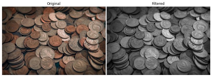
coins_3 = imread("images/coins_3.jpg")
# Convert to gray
coins_3_gray = rgb2gray(coins_3)
compare(coins_3, coins_3_gray)
要找到边缘,我们只需将图像传递给canny函数:
from skimage.feature import canny
# Find edges with canny
canny_edges = canny(coins_3_gray)
compare(coins_3, canny_edges, "Edges detected with Canny algorithm")
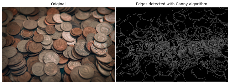
该算法发现了几乎所有硬币的边缘,但由于硬币上的雕刻也被检测到,因此噪声非常大。我们可以通过调整sigma参数来降低canny的灵敏度:
canny_edges_sigma_2 = canny(coins_3_gray, sigma=2.5)
compare(coins_3, canny_edges_sigma_2, "Edges detected with less intensity")
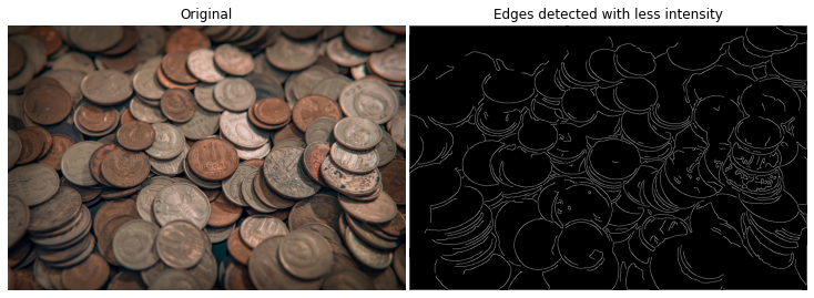
正如你所见,Canny现在只找到了硬币的大致轮廓。
2、角点检测
另一种重要的图像处理技术是角点检测。角点可以是图像分类中对象的关键特征。
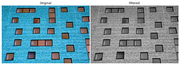
为了找到角点,我们将使用Harris角点检测算法。让我们加载一个示例图像并将其转换为灰度:
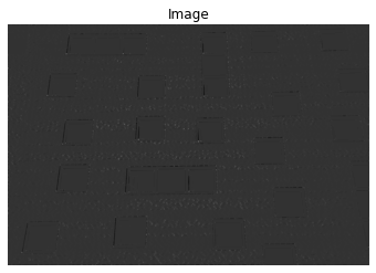
windows = imread("images/windows.jpg")
windows_gray = rgb2gray(windows)
compare(windows, windows_gray)
我们将使用corner_harris函数生成一个测量图像,该图像屏蔽了角点所在的区域。
from skimage.feature import corner_harris
measured_image = corner_harris(windows_gray)
>>> show(measured_image)
现在,我们将此蒙版度量图像传递给corner_peaks函数,该函数这次返回角点坐标:
from skimage.feature import corner_peaks
corner_coords = corner_peaks(measured_image, min_distance=50)
>>> len(corner_coords)
79
该函数找到79个角点。让我们将操作包装到函数中:
def find_corner_coords(image, min_distance=50):
# Convert to gray
gray_image = rgb2gray(image)
# Produce a measure image
measure_image = corner_harris(gray_image)
# Find coords
coords = corner_peaks(measure_image, min_distance=min_distance)
return coords
现在,我们将创建另一个函数,该函数使用上述函数生成的坐标绘制每个角点:
def show_image_cornered(image):
# Find coords
coords = find_corner_coords(image)
# Plot them on top of the image
plt.imshow(image, cmap="gray")
plt.plot(coords[:, 1], coords[:, 0], "+b", markersize=15)
plt.axis("off")
show_image_cornered(windows)
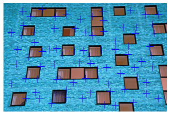
不幸的是,该算法没有按预期工作。标记放置在砖的交叉处,而不是找到窗角。
这些是噪音,使它们毫无用处。让我们对图像进行去噪处理,并再次将其传递给函数:
windows_denoised = denoise_tv_chambolle(windows, multichannel=True, weight=0.3)
show_image_cornered(windows_denoised)
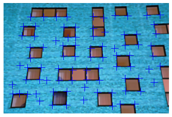
现在,这好多了!它找到了大部分窗户角。
结论
在真正的计算机视觉问题中,你不会同时使用所有这些。正如你可能已经注意到的,我们今天学到的东西并不复杂,最多需要几行代码。棘手的部分是将它们应用于实际问题,并实际提高模型的性能。
感谢阅读!