基于卷积神经网络的图像分类
现在是学习卷积神经网络及其在图像分类中的应用了。

什么是卷积?
卷积运算是使用具有恒定大小的“窗口”移动图像,并将图像像素与卷积窗口相乘以获得输出图像的过程。让我们看看下面的例子:

我们看到一个9x9图像和一个3x3卷积滤波器,其恒定权重为3 0 3 2 0 2 1 0 1,以及卷积运算的计算。尝试使用如下所示的滤波器遍历图像,并更好地了解输出图像的这些像素是如何通过卷积计算的。

窗口、滤波器、核、掩码是提到“卷积滤波器”的不同方式,我们也将在本文中使用这些术语。
填充
填充是在输入图像边框上添加额外像素的过程,主要是为了保持输出图像的大小与输入图像的大小相同。最常见的填充技术是添加零(称为零填充)。
跨步
步幅是我们使用卷积窗口遍历图像时每次迭代的步长。在下面的例子中,我们实际上看到步幅是1,所以我们将窗口移动了1。现在让我们看另一个例子,更好地理解水平步幅=1,垂直步幅=2:

因此,填充大小、步幅大小、滤波器大小和输入大小会影响输出图像的大小,根据这些不同的参数,输出图像大小的公式如下:

到目前为止,我们只研究了一个应用于输入图像的卷积运算,现在让我们看看什么是卷积神经网络,以及我们如何训练它们。
卷积神经网络(CNN)
如果将层作为卷积窗口,窗口中的每个像素实际上是一个权重(而不是我们在前一篇文章中学习的全连接的神经网络),那么这是一个卷积神经网络。
我们的目标是训练模型,以在最后以最小的成本更新这些权重。因此,与前面的例子相反,我们的卷积滤波器中没有任何常量值,我们应该让模型为它们找到最佳值。
所以一个简单的CNN是一些卷积运算的序列,如下所示:

基于CNN的图像分类
但是如何利用CNN实现图像分类呢?
图像分类的唯一区别是,我们现在处理的是图像,而不是房价、房间号等结构化数据。
每个卷积运算都会参与提取图像特征,例如耳朵、脚、狗的嘴等。随着卷积层的加深,该特征提取步骤会更深入,而在第一层,我们只获得图像的一些边缘。
因此,卷积层负责提取重要的特征,最后,为了有一个完整的图像分类模型,我们只需要一些全连接的输出节点,根据它们的权重来决定图像的正确类别!
我们假设狗有一个分类问题。在这种情况下,在训练结束时,一些输出节点将代表狗类特征和一些猫类特征。
如果通过这些卷积层的输入图像在激活函数结束时狗类提供了更高的值,那么他将分类为狗。否则分类为猫。让我们可视化一下这个过程:

CNN+全连接的神经网络创建了一个图像分类模型!
在讨论用于图像分类的常见CNN体系结构之前,让我们先来看一些更复杂、更真实的CNN示例:
当我们谈论CNN层时,我们并不是只讨论一层中的一个卷积核;实际上,多个卷积核可以创建一个卷积层。所以我们把所有这些卷积滤波器一个接一个地应用到我们的输入图像上,然后我们传递到下一个卷积层。1个卷积层中卷积核的数量有3个,与图像的“通道大小”相同。

我们学习了如何在应用卷积运算后计算输出图像大小,现在你应该知道卷积层的通道大小直接是输出通道大小,因为我们应用1个卷积运算来获得1个输出图像。因此,如果CNN层内部有5个卷积核,我们在这一层的末尾得到5个输出核。
如果我们使用RGB图像,我们有3个通道,而灰度图像有1个通道。在这种情况下,我们应用1个卷积核3次,以获得输出通道。因此,输出图像的通道大小不会改变,但卷积层的参数总数会改变。1个CNN层的参数总数计算如下:

因此,对于我们前面的例子,我们可以说n=64 m=64 l=1 k=32。
池化
这是图像分类中使用的另一个重要术语。这是一种用于减少CNN模型参数的方法。
逐次减少参数的数量,并且只从特征映射中选择最重要的特征(来自每个卷积层的输出映射。正如我们之前所说,更深的卷积层具有更具体的特征)是很重要的。有两种常见的池类型:
最大池
其基本思想是再次使用窗口,此时不使用任何权重,在遍历特征图时,选择最大像素值作为输出。

我们使用相同的公式来计算带有卷积运算的最大池的输出映射大小,正如我前面提到的。重要的一点是,由于其目的是减少参数大小,因此给定padding size=0和stride size=池内核的大小是一种合理且常用的方法,就像我们在本例中所做的那样。
平均池
我们不是根据最大像素计算输出,而是根据池内核中像素的平均值计算输出。

通用卷积神经网络结构
ImageNet大规模视觉识别挑战赛(ILSVRC)多年来一直是一项非常受欢迎的比赛。我们将考察不同年份该竞赛的一些获胜者。这些是图像分类任务中最常见的架构,与其他模型相比,它们具有更高的性能。
ImageNet是一个数据集,有1281167张训练图像、50000张验证图像和100000张1000个类的测试图像。
验证数据集:除了用于任何模型的训练步骤的训练数据集和训练步骤完成后用于测试模型的测试图像,以计算模型精度性能外,它是模型以前没有见过的数据,即在训练阶段不参与反向传播权重更新阶段,但用于测试,以便真实地跟踪训练阶段的进度。
· AlexNet (2012)
该模型由8层组成,5层卷积,3层全连接。
用于RGB输入图像(3通道)
包含6000万个参数
ImageNet测试数据集的最终误差为15.3%
该模型首次使用了ReLU激活函数。除了最后一个完全连接的层具有Softmax激活功能外,ReLu用作整个模型的激活功能
使用0.5%的Dropout。
使用动量为0.9且批量为128的随机梯度下降法
使用标准差=0.01的零平均高斯分布初始化权重
偏置以恒定值1初始化。
学习率初始化为0.01,“权重衰减正则化”应用为0.0005

在上图中,我们看到了AlexNet体系结构,我们有1000个完全连接层的节点,因为ImageNet数据集有1000个类。
在这个架构中,我们还遇到了一些我以前没有提到的术语:
动量梯度下降:这是对梯度下降计算的优化,我们将之前梯度下降的导数添加到我们的梯度下降计算中。我们用动量超参数乘以这个附加部分,对于这个架构,动量超参数是0.9。
高斯分布的权重初始化:在开始训练模型之前,有不同的方法初始化我们的权重。例如,将每个权重设为0是一种方法,但这是一种糟糕的方法!与此相反,根据高斯分布初始化所有权重是一种常用的方法。我们只需要选择分布的平均值和标准差,我们的权重将在这个分布范围内。
权重衰减优化:在本文中使用SGD(随机梯度下降)的情况下,L2正则化也是如此!
· VGG16(2014)
VGG架构是一个16层模型,具有13个卷积和3个全连接。
它有1.38亿个参数
测试数据集有7.5%的错误
与AlexNet相反,每个卷积层中的所有核都使用相同的大小。这是3x3的核,步幅=1,填充=1。最大池为2x2,步长=2
与AlexNet类似,ReLu用于隐藏层,Softmax用于输出层。动量为0.9的SGD,衰减参数为0.00005的权重衰减正则化,初始学习率为0.01,使用高斯分布的权重初始化。
作为AlexNet之间的一个小差异,VGG16体系结构使用批量大小=256,将偏差初始化为0,而不是1,并且具有224x224x3的输入图像大小。
有一个新版本名为VGG19,共有19层。
· ResNet(2015)
该架构的名称来自Residual Blocks,其中Residual Blocks是“输入”和“卷积和激活函数后的输出”的组合。

有不同版本的ResNet具有不同数量的层,如Resnet18、Resnet34、Resnet50、Resnet101和Resnet152。在下图中,我们在左侧看到一个“正常”的18层架构,在右侧看到ResNet版本。
红线表示它们具有相同的尺寸,因此可以直接组合,而蓝线表示尺寸不同,因此应使用零填充或在使用1x1卷积内核使用兼容的填充调整大小。

ResNet152实现了测试数据集的%3.57错误,它有58M个参数。当我们将参数大小和小误差与以前的架构进行比较时,效果很好,对吗?
除了可训练参数的数量外,浮点运算(每秒浮点运算)也是一个重要因素。让我们比较一下我们迄今为止研究的模型:

如果你想研究更多类型的卷积神经网络,建议你搜索Inception、SeNet(2017年ILSVRC获奖者)和MobileNet。
现在是我们将VGG16与Python和Tensorflow结合使用来应用图像分类的时候了!
VGG架构实现
# import necessary layers
from tensorflow.keras.layers import Input, Conv2D , Dropout, MaxPool2D, Flatten, Dense
from tensorflow.keras import Model
from tensorflow.keras.preprocessing.image import ImageDataGenerator
from tensorflow.keras.regularizers import l2
import tensorflow as tf
from tensorflow.keras.callbacks import EarlyStopping, ModelCheckpoint
import os
import matplotlib.pyplot as plt
import sys
from tensorflow.keras.callbacks import CSVLogger
MODEL_FNAME = "trained_model.h5"
base_dir = "dataset"
tmp_model_name = "tmp.h5"
INPUT_SIZE = 224
BATCH_SIZE = 16
physical_devices = tf.config.list_physical_devices()
print("DEVICES : ", physical_devices)
print('Using:')
print(' u2022 Python version:',sys.version)
print(' u2022 TensorFlow version:', tf.__version__)
print(' u2022 tf.keras version:', tf.keras.__version__)
print(' u2022 Running on GPU' if tf.test.is_gpu_available() else ' u2022 GPU device not found. Running on CPU')
count = 0
previous_acc = 0
if not os.path.exists(MODEL_FNAME):
""" Create VGG Model"""
# input
input = Input(shape =(INPUT_SIZE,INPUT_SIZE,3))
weight_initializer = tf.keras.initializers.RandomNormal(mean=0.0, stddev=0.01, seed=None)
bias_initializer=tf.keras.initializers.Zeros()
# 1st Conv Block
x = Conv2D (filters =64, kernel_size =3, padding ='same', activation='relu',kernel_initializer=weight_initializer,kernel_regularizer=l2(0.00005),bias_initializer=bias_initializer)(input)
x = Conv2D (filters =64, kernel_size =3, padding ='same', activation='relu',kernel_initializer=weight_initializer,kernel_regularizer=l2(0.00005),bias_initializer=bias_initializer)(x)
x = MaxPool2D(pool_size =2, strides =2, padding ='same')(x)
# 2nd Conv Block
x = Conv2D (filters =128, kernel_size =3, padding ='same', activation='relu',kernel_initializer=weight_initializer,kernel_regularizer=l2(0.00005),bias_initializer=bias_initializer)(x)
x = Conv2D (filters =128, kernel_size =3, padding ='same', activation='relu',kernel_initializer=weight_initializer,kernel_regularizer=l2(0.00005),bias_initializer=bias_initializer)(x)
x = MaxPool2D(pool_size =2, strides =2, padding ='same')(x)
# 3rd Conv block
x = Conv2D (filters =256, kernel_size =3, padding ='same', activation='relu',kernel_initializer=weight_initializer,kernel_regularizer=l2(0.00005),bias_initializer=bias_initializer)(x)
x = Conv2D (filters =256, kernel_size =3, padding ='same', activation='relu',kernel_initializer=weight_initializer,kernel_regularizer=l2(0.00005),bias_initializer=bias_initializer)(x)
x = Conv2D (filters =256, kernel_size =3, padding ='same', activation='relu',kernel_initializer=weight_initializer,kernel_regularizer=l2(0.00005),bias_initializer=bias_initializer)(x)
x = MaxPool2D(pool_size =2, strides =2, padding ='same')(x)
# 4th Conv block
x = Conv2D (filters =512, kernel_size =3, padding ='same', activation='relu',kernel_initializer=weight_initializer,kernel_regularizer=l2(0.00005),bias_initializer=bias_initializer)(x)
x = Conv2D (filters =512, kernel_size =3, padding ='same', activation='relu',kernel_initializer=weight_initializer,kernel_regularizer=l2(0.00005),bias_initializer=bias_initializer)(x)
x = Conv2D (filters =512, kernel_size =3, padding ='same', activation='relu',kernel_initializer=weight_initializer,kernel_regularizer=l2(0.00005),bias_initializer=bias_initializer)(x)
x = MaxPool2D(pool_size =2, strides =2, padding ='same')(x)
# 5th Conv block
x = Conv2D (filters =512, kernel_size =3, padding ='same', activation='relu',kernel_initializer=weight_initializer,kernel_regularizer=l2(0.00005),bias_initializer=bias_initializer)(x)
x = Conv2D (filters =512, kernel_size =3, padding ='same', activation='relu',kernel_initializer=weight_initializer,kernel_regularizer=l2(0.00005),bias_initializer=bias_initializer)(x)
x = Conv2D (filters =512, kernel_size =3, padding ='same', activation='relu',kernel_initializer=weight_initializer,kernel_regularizer=l2(0.00005),bias_initializer=bias_initializer)(x)
x = MaxPool2D(pool_size =2, strides =2, padding ='same')(x)
# Fully connected layers
x = Flatten()(x)
x = Dropout(0.5)(x)
x = Dense(units = 4096, activation ='relu', kernel_initializer=weight_initializer,kernel_regularizer=l2(0.00005),bias_initializer=bias_initializer)(x)
x = Dropout(0.5)(x)
x = Dense(units = 4096, activation ='relu', kernel_initializer=weight_initializer,kernel_regularizer=l2(0.00005),bias_initializer=bias_initializer)(x)
output = Dense(units = 2, activation ='softmax')(x)
# creating the model
model = Model (inputs=input, outputs =output)
m = model
m.save(tmp_model_name)
del m
tf.keras.backend.clear_session()
model.summary()
""" Prepare the Dataset for Training"""
train_dir = os.path.join(base_dir, 'train')
val_dir = os.path.join(base_dir, 'validation')
train_batches = ImageDataGenerator(rescale = 1 / 255.).flow_from_directory(train_dir,
target_size=(INPUT_SIZE,INPUT_SIZE),
shuffle=True,
seed=42,
batch_size=BATCH_SIZE)
val_batches = ImageDataGenerator(rescale = 1 / 255.).flow_from_directory(val_dir,
target_size=(INPUT_SIZE,INPUT_SIZE),
shuffle=True,
seed=42,
batch_size=BATCH_SIZE)
""" Train """
class CustomLearningRateScheduler(tf.keras.callbacks.Callback):
def __init__(self, schedule):
super(CustomLearningRateScheduler, self).__init__()
self.schedule = schedule
def on_epoch_end(self, epoch, logs=None):
if not hasattr(self.model.optimizer, "lr"):
raise ValueError('Optimizer must have a "lr" attribute.')
# Get the current learning rate from model's optimizer.
lr = float(tf.keras.backend.get_value(self.model.optimizer.learning_rate))
# Call schedule function to get the scheduled learning rate.
# keys = list(logs.keys())
# print("keys",keys)
val_acc = logs.get("val_binary_accuracy")
scheduled_lr = self.schedule(lr, val_acc)
# Set the value back to the optimizer before this epoch starts
tf.keras.backend.set_value(self.model.optimizer.lr, scheduled_lr)
def learning_rate_scheduler(lr, val_acc):
global count
global previous_acc
if val_acc == previous_acc:
# print("acc ", val_acc, "previous acc ", previous_acc)
count += 1
else:
count = 0
if count >= 5:
print("acc is the same for 10 epoch, learnin rate decreased by /10")
count = 0
lr /= 10
print("new learning rate:", lr)
previous_acc = val_acc
return lr
#compile the model by determining loss function Binary Cross Entropy, optimizer as SGD
model.compile(optimizer=tf.keras.optimizers.SGD(lr=0.0000001, momentum=0.9),
loss=tf.keras.losses.BinaryCrossentropy(),
metrics=[tf.keras.metrics.BinaryAccuracy()],
sample_weight_mode=[None])
early_stopping = EarlyStopping(monitor='val_loss', patience=10)
checkpointer = ModelCheckpoint(filepath=MODEL_FNAME, verbose=1, save_best_only=True)
csv_logger = CSVLogger('log.csv', append=True, separator=' ')
history=model.fit(train_batches,
validation_data = val_batches,
epochs = 100,
verbose = 1,
shuffle = True,
callbacks = [checkpointer,early_stopping,CustomLearningRateScheduler(learning_rate_scheduler),csv_logger])
""" Plot the train and validation Loss """
plt.plot(history.history['loss'])
plt.plot(history.history['val_loss'])
plt.title('model loss')
plt.ylabel('loss')
plt.xlabel('epoch')
plt.legend(['train', 'validation'], loc='upper left')
plt.show()
""" Plot the train and validation Accuracy """
plt.plot(history.history['binary_accuracy'])
plt.plot(history.history['val_binary_accuracy'])
plt.title('model accuracy')
plt.ylabel('accuracy')
plt.xlabel('epoch')
plt.legend(['train', 'validation'], loc='upper left')
plt.show()
print("End of Training")
else:
""" Test """
test_dir = os.path.join(base_dir, 'test')
test_batches = ImageDataGenerator(rescale = 1 / 255.).flow_from_directory(test_dir,
target_size=(INPUT_SIZE,INPUT_SIZE),
class_mode='categorical',
shuffle=False,
seed=42,
batch_size=1)
model = tf.keras.models.load_model(MODEL_FNAME)
model.summary()
# Evaluate on test data
scores = model.evaluate(test_batches)
print("metric names",model.metrics_names)
print(model.metrics_names[0], scores[0])
print(model.metrics_names[1], scores[1])
tf.keras.backend.clear_session()
这是使用Python和Tensorflow实现的VGG16。让我们稍微检查一下代码
· 首先,我们检查我们的TensorFlow Cuda Cudnn安装是否正常,以及TensorFlow是否可以找到我们的GPU。因为如果不是这样的话,那就意味着有一个包冲突或一个错误,我们应该解决,因为使用CPU进行模型训练太慢了。
· 然后,我们使用Conv2D函数为卷积层创建VGG16模型,MaxPool2D函数为最大池层,展平函数为CNN输出一个能够传递到全连接层的展平输入,Dense函数为全连接层,Dropout函数为最后一个全连接层之间添加Dropout优化。可以看到,我们应该在使用相关层函数的同时,将权重初始化、偏差初始化、l2正则化器1x1添加到层中。请注意,正态分布是高斯分布的同义词,所以当看到weight_initializer = tf.keras.initializers.RandomNormal(mean=0.0, stddev=0.01, seed=None),不要困惑
· 将用两个类来测试这个模型,而不是用1000个类来测试巨大的ImageNet数据集,所以我将输出层从1000个节点更改为2个节点
· 使用ImageGenerator函数和flow_from_directory,我们将数据集准备为能够使用TensorFlow模型的向量。我们这里也给出了批量大小。(由于我的电脑内存不足,我可以给出16个,而不是论文中提到的256个。shuffle参数意味着数据集将在每个epoch前被打乱
· model.compile()函数是训练模型之前的最后一部分。我们决定使用哪个优化器(带动量的SGD)、哪个损失函数(因为在我们的例子中我们有两个类),以及在训练期间计算性能的指标(二进制精度)。
· 使用model.fit()训练我们的模型。添加了一些选项,比如“EarlyStoping”和“ModelCheckPoint”回调。如果验证损失在10个epoch内没有增加,则第一个epoch停止训练,如果验证损失比前一epoch好,则模型检查点不仅在最后保存我们的模型,而且在训练期间保存我们的模型。
· CustomLearningRateScheduler是我手动实现的学习速率调度器,用于应用“如果验证准确率停止提高,我们将通过除以10来更新学习速率”
· 在训练结束时,我将验证和训练数据集的准确性和损失图可视化。
· 最后一部分是使用测试数据集测试模型。我们检查是否有任何名为“trained_model.h5”的训练模型,如果没有,我们训练一个模型,如果有,我们使用这个模型来测试性能
想解释一下我在解释代码时使用的一些术语:
· 验证集准确率:验证集准确率是一种衡量模型在验证数据集上表现的指标。它只是检查在验证数据集中有多少图像预测为真。我们也会对训练数据集进行同样的检查。但这只是为了我们监控模型,只有训练损失用于梯度下降计算
· 迭代-epoch:1迭代是为一批中的所有图像提供模型的过程。Epoch是指为训练数据集中的所有图像提供模型的过程。例如,如果我们有100张图片,batch=10,那么1个epoch将有10次迭代。
· 展平:这只不过是重塑CNN输出,使其具有1D输入,这是从卷积层传递到全连接层的唯一方法。
· 现在让我们检查一下结果

即使通过监控验证准确度来改变学习率,结果也不是很好,验证准确度也没有提高。但是为什么它不能像VGG16论文中那样直接工作呢?
1. 在最初的论文中,我们讨论了374个epoch的1000个输出类和1500000个图像。不幸的是,使用这个数据集并训练1000个类的模型需要几天的时间,所以正如我之前所说,我使用了两个类的数据集,并将输出层更改为有两个输出节点。
1. 模型体系结构和数据集都需要不同的优化,因此一个运行良好的模型可能不适用于另一个数据集。
3. 微调超参数以改进模型与首先了解如何构建模型一样重要。你可能已经注意到我们需要微调多少超参数
· 权重和偏差初始化
· 损失函数选择
· 初始学习率选择
· 优化器选择(梯度下降法)
· Dropout与否的使用
· 数据扩充(如果你没有足够的图像,或者它们太相似,你希望获得相同图像的不同版本)
等等…
但在你对如何优化这么多变量感到悲观之前,想提两点。
1.迁移学习
这是一种非常重要的方法,我们使用预先训练好的模型,用我们自己的数据集对其进行训练。在我们的例子中,我们不会只使用VGG16体系结构,而是一个已经使用VGG16体系结构和ImageNet数据集训练过的模型,我们将使用比ImageNet小得多的数据集对其进行重新训练。
这种方法为我们提供了一个并非未知的起点——一些随机权重。我们的数据集可能包含不同的对象,但不同对象之间有一些基本的共同特征,比如边、圆形,为什么不使用它们,而不是从头开始呢?我们将看到这种方法如何减少耗时并提高精度性能。
2.当查看我们的输出时,发现问题不是因为模型停止学习,而是因为它没有开始学习!精度从0.5开始,没有改变!这个具体的结果给了我们一个非常明确的信息:我们应该降低学习率,让模型开始学习。请记住,学习率是学习的步长,每次迭代的梯度下降计算会对权重产生多大影响。如果这个速率太大,步骤太大,我们无法控制权重更新,因此模型无法学习任何东西。
以下代码仅包括迁移学习的更改,其中采用了带有预训练权重Tensorflow内置模型和较低学习率(0.001)的模型
# -*- coding: utf-8 -*-
"""
Created on Wed Dec 29 20:56:04 2021
@author: aktas
"""
# import necessary layers
from tensorflow.keras.preprocessing.image import ImageDataGenerator
from tensorflow.keras.regularizers import l2
import tensorflow as tf
from tensorflow.keras.callbacks import EarlyStopping, ModelCheckpoint
import os
import matplotlib.pyplot as plt
import sys
from tensorflow.keras.callbacks import CSVLogger
from tensorflow.keras.applications import vgg16, imagenet_utils
from tensorflow.keras.layers import Dense, Flatten
from tensorflow.keras.models import Model
MODEL_FNAME = "pretrained_model.h5"
tmp_model_name = "tmp.h5"
base_dir = "dataset"
INPUT_SIZE = 224
BATCH_SIZE = 16
physical_devices = tf.config.list_physical_devices()
print("DEVICES : ", physical_devices)
print('Using:')
print(' u2022 Python version:',sys.version)
print(' u2022 TensorFlow version:', tf.__version__)
print(' u2022 tf.keras version:', tf.keras.__version__)
print(' u2022 Running on GPU' if tf.test.is_gpu_available() else '
u2022 GPU device not found. Running on CPU')
count = 0
previous_acc = 0
if not os.path.exists(MODEL_FNAME):
base_model = vgg16.VGG16(weights='imagenet', include_top=False, input_shape=(INPUT_SIZE,INPUT_SIZE,3))
m = base_model
m.save(tmp_model_name)
del m
tf.keras.backend.clear_session()
print("Number of layers in the base model: ", len(base_model.layers))
base_model.trainable = False
last_output = base_model.output
x = Flatten()(last_output)
x = Dense(2, activation='softmax')(x)
model = Model(inputs=[base_model.input], outputs=[x])
model.summary()
""" Prepare the Dataset for Training"""
train_dir = os.path.join(base_dir, 'train')
val_dir = os.path.join(base_dir, 'validation')
train_batches = ImageDataGenerator(rescale = 1 / 255.).flow_from_directory(train_dir,
target_size=(INPUT_SIZE,INPUT_SIZE),
shuffle=True,
seed=42,
batch_size=BATCH_SIZE)
val_batches = ImageDataGenerator(rescale = 1 / 255.).flow_from_directory(val_dir,
target_size=(INPUT_SIZE,INPUT_SIZE),
shuffle=True,
seed=42,
batch_size=BATCH_SIZE)
""" Train """
class CustomLearningRateScheduler(tf.keras.callbacks.Callback):
def __init__(self, schedule):
super(CustomLearningRateScheduler, self).__init__()
self.schedule = schedule
def on_epoch_end(self, epoch, logs=None):
if not hasattr(self.model.optimizer, "lr"):
raise ValueError('Optimizer must have a "lr" attribute.')
# Get the current learning rate from model's optimizer.
lr = float(tf.keras.backend.get_value(self.model.optimizer.learning_rate))
# Call schedule function to get the scheduled learning rate.
# keys = list(logs.keys())
# print("keys",keys)
val_acc = logs.get("val_binary_accuracy")
scheduled_lr = self.schedule(lr, val_acc)
# Set the value back to the optimizer before this epoch starts
tf.keras.backend.set_value(self.model.optimizer.lr, scheduled_lr)
def learning_rate_scheduler(lr, val_acc):
global count
global previous_acc
if val_acc <= previous_acc:
# print("acc ", val_acc, "previous acc ", previous_acc)
count += 1
else:
previous_acc = val_acc
count = 0
if count >= 5:
print("acc is the same for 10 epoch, learnin rate decreased by /10")
count = 0
lr /= 10
print("new learning rate:", lr)
return lr
#compile the model by determining loss function Binary Cross Entropy, optimizer as SGD
model.compile(optimizer=tf.keras.optimizers.SGD(lr=0.001, momentum=0.9),
loss=tf.keras.losses.BinaryCrossentropy(),
metrics=[tf.keras.metrics.BinaryAccuracy()],
sample_weight_mode=[None])
early_stopping = EarlyStopping(monitor='val_loss', patience=10)
checkpointer = ModelCheckpoint(filepath=MODEL_FNAME, verbose=1, save_best_only=True)
csv_logger = CSVLogger('log.csv', append=True, separator=' ')
history=model.fit(train_batches,
validation_data = val_batches,
epochs = 100,
verbose = 1,
shuffle = True,
callbacks = [checkpointer,early_stopping,CustomLearningRateScheduler(learning_rate_scheduler),csv_logger])
""" Plot the train and validation Loss """
plt.plot(history.history['loss'])
plt.plot(history.history['val_loss'])
plt.title('model loss')
plt.ylabel('loss')
plt.xlabel('epoch')
plt.legend(['train', 'validation'], loc='upper left')
plt.show()
""" Plot the train and validation Accuracy """
plt.plot(history.history['binary_accuracy'])
plt.plot(history.history['val_binary_accuracy'])
plt.title('model accuracy')
plt.ylabel('accuracy')
plt.xlabel('epoch')
plt.legend(['train', 'validation'], loc='upper left')
plt.show()
print("End of Training")
else:
""" Test """
test_dir = os.path.join(base_dir, 'test')
test_batches = ImageDataGenerator(rescale = 1 / 255.).flow_from_directory(test_dir,
target_size=(INPUT_SIZE,INPUT_SIZE),
class_mode='categorical',
shuffle=False,
seed=42,
batch_size=1)
model = tf.keras.models.load_model(MODEL_FNAME)
model.summary()
# Evaluate on test data
scores = model.evaluate(test_batches)
print("metric names",model.metrics_names)
print(model.metrics_names[0], scores[0])
print(model.metrics_names[1], scores[1])
tf.keras.backend.clear_session()
让我们检查一下结果:


性能有了很大的提高,对吧?!我们看到,验证精度不再被卡住,直到0.97,而训练精度达到1.00。

一切似乎都很好!
想和大家分享我做的一些实验及其结果:
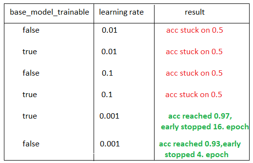
现在,我们可以做以下分析:
如果我们有一个不兼容的学习率,迁移学习本身仍然是不够的。
如果我们将base_model_trainable变量设置为False,这意味着我们不训练我们所使用的模型,我们只训练我们添加的最后一个全连接层。(VGG有1000个输出,所以我使用include_top=False不使用最后的全连接层,并且我在这个预训练模型的末尾添加了一个自己的全连接层,正如我们在代码中看到的那样)
从零开始改变了vgg_from_scratch实现的学习率,但validation 准确率仍然停留在0.5上,所以仅仅优化学习率本身是不够的。(至少如果你没有时间在微调后从头开始训练模型。)
可以通过此链接访问使用的数据集,请不要忘记将其与下面的代码放在同一文件夹中(当然,训练完成后,.h和日志文件会出现!????):
https://drive.google.com/drive/folders/1vt8HiybDroEMCvpdGQJx2T50Co4nZNYe?usp=sharing
使用Anaconda和Python=3.7、Tensorflow=2.2.0、Cuda=10.1、Cudnn=7.6.5来使用GPU训练和测试我的模型。如果你不熟悉这些术语,这里有一个快速教程:
下载Anaconda(请为你的计算机选择正确的系统)
打开Anaconda terminal,并使用conda create-n im_class python=3.7 Anaconda命令创建环境。环境可能是Anaconda最重要的属性,它允许你为不同的项目单独工作。你可以将任何包添加到你的环境中,如果你需要另一个包的另一个版本,你可以简单地创建另一个环境,以避免另一个项目崩溃,等等。
使用conda activate im_class命令进入你的环境以添加更多包(如果你忘记了这一步,你基本上不会对你的环境进行更改,而是在所有anaconda空间中进行更改)
使用pip install Tensorflow GPU==2.2.0安装具有GPU功能的Tensorflow
使用conda Install cudatoolkit=10.1命令安装CUDA和Cudnn
现在,你已经准备好测试上述代码了!
请注意,软件包版本之间的冲突是一个巨大的问题。这将帮助你在构建环境时花费更少的时间。
你已经完成了卷积神经网络图像分类教程。你可以尝试从头开始构建任何模型(甚至可能是你自己的模型)对其进行微调,针对不同的体系结构应用迁移学习,等等。
参考引用